long-reads-workshop
Now that we have a decent draft assembly for our bacterial isolate we can start to annotate the sequence. Annotation is ultimately about providing biological interpretation onto what is otherwise just a bare and uninteresting sequence of letters.
One thing to note is that in general bacterial annotation is simpler and more reliable than for Eukaryotes. This is largely because Eukaryotic genes contain introns which vastly complicates the process of correctly finding coding sequences and how these relate to units of expression (genes).
Genome Annotation
Prokka is an extremely fast and widely used bacterial genome annotation pipeline.
One of the key features of Prokka is its hierarchical approach to annotation. This allows it to be fast and sensitive as well as preferentially using more reliable information.
The process goes something like this.
- Find the locations of genes and their coding sequences
- Describe gene functions by comparing the coding sequence with databases of sequences with known function as follows;
- Proteins in Uniprot with protein or transcript evidence (reliable genes)
- All proteins in RefSeq from bacteria with finished genomes (unknown but well assembled)
- Databases of conserved protein domains (eg PFam)
- Predict other genomic features using additional tools;
- RNAmmer to find rRNA
- Aragorn to find tRNA
- Infernal to find ncRNA
Install Prokka
Fortunately prokka is available through conda so installation is very easy
conda create -n prokka prokka
conda activate prokka
Run Prokka
Create a directory for running prokka (as we have done for all other steps)
cd ~/nanopore_workshop
mkdir prokka
Create a symbolic link to the assembly we wish to annotate. In this case we will use the flye_20x assembly from Tuesday. It is not as nice as the polished medaka assembly but it is fairly close. More importantly the raw flye assembly contains all the original contigs and has associated information (eg the assembly graph) that we will exploit later in this tutorial.
cd prokka
ln -s ../quast/medaka/vibrio.fasta .
prokka --outdir vibrio --prefix vibrio vibrio.fasta
Now take a look inside the output directory created by prokka
ls vibrio
There are lots of files. This is because prokka anticipates the need to have annotation information in a variety for formats.
Explore the outputs as follows;
Proteins
head -n 20 vibrio/vibrio.faa
How many predicted proteins are there?
grep '>' vibrio/vibrio.faa | wc -l
Transcripts
head -n 20 vibrio/vibrio.ffn
How many predicted transcripts are there?
grep '>' vibrio/vibrio.ffn | wc -l
Question?: There are more predicted transcripts than proteins. Why might that be?
One way to answer this question might be to look at the names of sequences that exist in the ffn file that do not exist in the faa file. Luckily prokka uses identical names for transcripts and their protein products so we can find the differences easily using a unix tool called diff
diff <(grep '>' vibrio/vibrio.ffn) <(grep '>' vibrio/vibrio.faa)
Features
The gff and gbk files produced by prokka provide details of each feature (eg a gene) and its coordinates in the genome file.
Take a look at the first few lines of the gff file.
head vibrio/vibrio.gff
Now look up the specifications for gff format at https://asia.ensembl.org/info/website/upload/gff3.html and use this to understand the gff file for our vibrio genome.
The gbk file contains similar information but is formatted in genbank format. One of the nice things about prokka is that it includes all the files that you would need to submit your annotated genome to genbank
head -n 50 vibrio/vibrio.gbk
Metabolic Activity
Another useful file produced by prokka is the .tsv file. This file is just a table (tab separated) with useful information about each gene. Where possible it includes a gene name and COG (for conserved genes) and an EC number (Enzyme Commission number).
The Vibrio genus is quite large and diverse but many strains have been found to be pathogenic. Something that might be of interest therefore would be to look at toxin genes. We could do a simple text search for these;
grep 'toxin' vibrio/vibrio.tsv
Mystery Repeat Region
On tuesday we used bandage to view the flye assembly and found that it contained a repeat region that could not be completely resolved.
We will revisit this today and use some additional analysis to figure out exactly what this repeat is and how where it exists in the genome.
Extract repeat region sequence
Use bandage to extract the repeat region as follows;
- Click on the repeat to select it
- Use the
Outputmenu to copy the repeat sequence to your clipboard - In rstudio, open a new blank text file and paste in the sequence
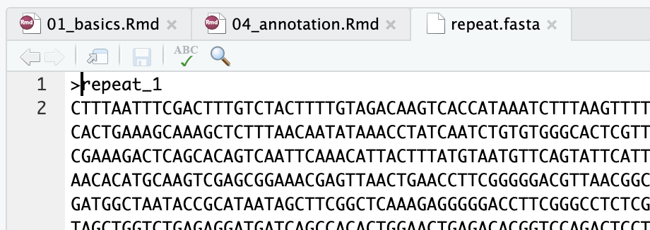
- Edit the text file to add a fasta header line (see below) with the text
>repeat_1 - Save the file into
prokka/repeat.fasta
Use prokka to annotate it
Now run prokka on this sequence to see if it contains any transcribed sequences
cd ~/nanopore_workshop/prokka/
prokka --outdir repeat --prefix repeat repeat.fasta
Now look at the tsv file that is produced. What type of genomic features dominate this sequence?
cat repeat/repeat.tsv
Genomic arrangement of repeats
Now we know the genes that are present in our repeat but we don’t know how the repeats are arranged in the genome. Specifically we are interested in whether they are arranged in tandem or dispersed throughout the genome.
To investigate this we can map the repeat sequence back to the genome itself. The tool of choice for mapping long reads and/or long DNA sequences is minimap2
Install minimap2
As usual this can be done with conda. Since minimap2 is a highly versatile tool, and since it has very few dependencies (unlikely to cause conflicts) we install it in our base environment.
conda activate base
conda install minimap2
Run the alignment
Previously we named our working directories after special tools that we used. This time the tool is very commonly used so we name the directory after what we are doing.
cd ~/nanopore_workshop
mkdir repeat_align
cd repeat_align
Link in the data
ln -s ../prokka/repeat.fasta .
ln -s ../prokka/vibrio.fasta .
Run minimap2. There are many ways to run minimap2. A great resource to help figure out which options to use is the minimap2 cookbook. In this case we are using minimap2 in much the same way as we would use to map reads.
minimap2 -x map-ont vibrio.fasta repeat.fasta > repeat_vs_genome.paf
Examine the alignment
Try looking at the first few lines of the paf file that was produced.
head repeat_vs_genome.paf
It looks complicated but is just another tab separated format. The format is described on this webpage. The first 12 columns are standard but more columns may be present (documented elsewhere).
For our purposes the important columns are those specifying the start and end point on the target. We can extract these columns into a bed formatted file as follows;
cat repeat_vs_genome.paf | grep '^repe' | awk -F '\t' '{print $6,$8,$9}' > repeat_locations.bed
We can get a quick idea of where these are spaced in the genome by using the ggbio package.
Installing and loading the required packages take a long time unfortunately
Caution: Run this during a break
if (!requireNamespace("BiocManager", quietly = TRUE))
    install.packages("BiocManager")

BiocManager::install("ggbio")
BiocManager::install("GenomicRanges")
BiocManager::install("rtracklayer")

library(ggbio)
library(GenomicRanges)
library(rtracklayer)
bed<-import("repeat_align/repeat_locations.bed")
autoplot(bed,chr.weight=1)
Question?: Is this a tandem repeat or interspersed?
Read Coverage in Repeat Regions
As a final component of examining the repeat in this genome we will investigate why this shows up with such high coverage in the assembly.
Begin by mapping all the reads to the flye_20x genome. Continue working from within the repeat_align directory.
ln -s ../flye/amtp4_20x.fastq .
This time we will get minimap2 to produce outputs in the sam format and then we will use samtools to compress this to bam. The sam format is a very widely used format for storing sequence alignment data and is much older than paf.
The reason we are converting to sam and then bam is that this will allow us to work with existing tool such as samtools and IGV.
Install samtools into the base conda environment
conda activate base
conda install samtools
minimap2 -a -x map-ont vibrio.fasta amtp4_20x.fastq | samtools view -b - > vibrio.amtp4.bam
Check that it worked by inspecting the first few lines using samtools view
samtools view vibrio.amtp4.bam | head
Ultimately we would like to visualise these alignments with IGV. In order to do this we need to sort and then index the alignments
samtools sort vibrio.amtp4.bam > vibrio.amtp4.sorted.bam
samtools index vibrio.amtp4.sorted.bam
Visualise alignments with IGV
Download IGV from https://software.broadinstitute.org/software/igv/ and install it on your laptop.
Then download the entire repeat_align folder from rstudio to your laptop.
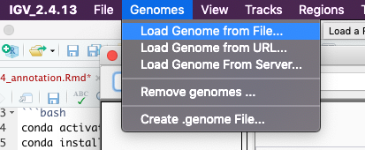
Once you have IGV working you should first load the genome file vibrio.fasta using the menu “Genomes” -> “Load from File”
You won’t see much after loading the genome because all you have available are the backbone genomic sequences.
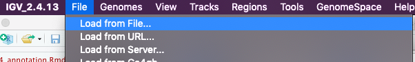
Next load the reads. You do this using “File” -> “Load from file”
Now zoom in on a random region to see some reads
Inspect read coverage in repeat regions
Now load the file repeat_locations.bed. If you are sufficiently zoomed out you should see these as a new track.
Try looking at a few of these regions and take note of the read coverage.
Do all the repeat regions have higher coverage? or just a few? Where do these extra reads come from?
Use samtools to filter alignments
Now go back to Rstudio and back to the repeat_align directory. From here we will use samtools to filter alignments to remove all Secondary alignments.
samtools view -b -F 256 vibrio.amtp4.sorted.bam >vibrio.amtp4.sorted.nosecondary.bam
samtools index vibrio.amtp4.sorted.nosecondary.bam
Download both these new files (the nosecondary.bam and its index) to your laptop and load them into IGV.
Look around at the repeat regions again. Compare coverage in the repeat regions between the filtered and unfiltered alignment files.
What does this tell us about how Flye is reporting read coverage in its assembly graph?
Optional: Load Gene GFF File into IGV
Download the prokka/vibrio/vibrio.gff file and load it into IGV.
Explore the genome. Try mousing over various features to see what information is displayed?
Note that IGV can navigate to specific regions or directly to genes.
GC Content
Variation in GC content is often a good way of detecting contigs in the assembly that come from very different taxa (eg as contaminants). There are many ways to calculate GC content. Here we will do it with a simple awk script that calculates a value every 100 base pairs
Start by creating a working directory for gc analysis
cd ~/nanopore_workshop
mkdir gc
cd gc
Create a new text file in rstudio and paste the following script into it
BEGIN {
  printf("contig\tgc\n")
}
$1 ~ /^>/ {
  contig=substr($1,2,9)
  position=0
  GC["A"]=0
  GC["T"]=0
  GC["G"]=0
  GC["C"]=0
  next
}

{
  split(toupper($0),seq,"")


  for(i in seq){
    b = seq[i]
    GC[b]++
    position+=1
    if ( position%100 == 0 ){
      gc_ratio = (GC["G"]+GC["C"])/(GC["A"]+GC["T"]+GC["G"]+GC["C"])
      printf("%s\t%s\n",contig, gc_ratio)
    }
  }
}
Save the script and name it gcwindow.awk. Be sure to save this into the gc directory you just created.
Now run the script on the flye assembly
ln -s ../flye/amtp4_20x/assembly.fasta flye20x.fasta
cat flye20x.fasta | awk -f gcwindow.awk > flye20x.gc.tsv
Now read the data into R and use ggplot to visualise it
gc <- read_tsv("gc/flye20x.gc.tsv")
ggplot(gc,aes(x=gc)) + geom_density(aes(color=contig))
Although this plot shows differences in GC content fairly well the colour scale makes it hard to see which contigs are which. Remember that the main Vibrio contigs are contig_3 and contig_16 .
Activity: Summarise gc for each contig by taking the mean value
gc_av <- gc %>% group_by(contig) %>%
    summarise(mean_gc = mean(gc))
We can look at this directly and we can also use it to add labels to our original plot. Before doing this install the ggrepel package.
ggplot(gc,aes(x=gc)) + geom_density(aes(color=contig)) + geom_label_repel(data = gc_av,aes(x=mean_gc,y=200,label=contig)) + coord_flip()
Whole genome alignments
Whole genome alignment is a good way to identify structural rearrangements between genomes of related species.
A good tool for this is D Genies
As an example of the use of this tool we will align the flye assembly to the published genome of Vibrio tubiashii, which is very closely related to our target and Vibrio choleriae which is more distant.
Download the genomes from genbank
Try aligning each of these against the Flye 20x assembly.
How does relatedness affect these types of plots? Take care to interpret the alignments correctly. In circular genomes a difference in coordinate starting point can lead to artifacts in the alignment plot.